> restart: with(plots):

> logplot( {exp(x), exp(x^2), exp(2*x)}, x=0.1..10, 1..10^6);

>

> s:= I*omega:

> f:= (1+s*2/5) * (1+s/9) / ( (1+s) * (1+s/99) ):

> setoptions(color=black):

> loglogplot( abs(f), omega=0.01..10000);

>

> loglogplot( abs(f), omega=0.01..10000, sample=[seq(10^(n/10), n=-20..50)], axes=boxed);

>

> semilogplot( argument(f)*180/Pi, omega=0.01..10000, sample=[seq(10^(n/10), n=-20..50)], axes=boxed);

>

>

> restart:

> with(plots):

Warning, the name changecoords has been redefined

> f:=(x-1)*(x+2)*(y-2)*(y+2):

> densityplot(f, x=-3..3, y=-3..3, axes=boxed);

> contourplot(f, x=-3..3, y=-3..3, color=black);

> contourplot(f, x=-3..3, y=-3..3,

> grid=[30,30], contours=25, color=black, axes=boxed);

> contourplot(f, x=-3..3, y=-3..3,

> axes=boxed, filled=true, coloring=[white,black]);

> contourplot3d(f, x=-3..3, y=-3..3,

> axes=boxed, filled=true, coloring=[white,black], shading=none);

>

> s:='s': grey75:=COLOR(RGB,.75,.75,.75):

> contourplot3d( [t*sin(s), t*cos(s),

> sin(s*t)], s=0..2*Pi, t=0..2, contours=20,

> filled=true, coloring=[white,grey], shading=none, orientation=[0,0]);

>

>

2D

> complexplot(tan(x*(1+I)), x=-Pi..Pi, color=black);

>

> solve(x^12=1);

> complexplot( [%], style=point, axes=boxed, thickness=3, color=black);

>

>

3D

> with(plots):

> complexplot3d(sin(z), z=-I..2*Pi+I, orientation=[-70,21], axes=boxed, style=patch, grid=[40,40]);

> f:=sin(z):

> complexplot3d( [Re(f),abs(f)], z=0..Pi+I, style=patch, axes=boxed);

> restart: with(plots):

Warning, the name changecoords has been redefined

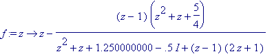
> p:=(z-1)*(z^2+z+5/4);

> f := unapply(z- p / (diff(p,z)-0.5*I), z);

>

> st:=time();

> complexplot3d(f@@4,-4-4*I..4+4*I,view=-1..2,style=patchnogrid,grid=[100,100]);

> time()-st;

>

>

>

>

>

Konforme Abbildungen

> with(plots):

> conformal(z, z=-1-I..2+I, axes=boxed);

> conformal(1/z, z=-1-I..2+I, axes=boxed);

> conformal(1/z, z=-1-I..2+I, -4-3*I..4+3*I, grid=[50,50], axes=boxed);

> #display(conformal(1/z, z=-1-I..2+I, -4-3*I..4+3*I, grid=[50,50], axes=boxed, #color=black), view=[-4..4, -3..3]);

>

> conformal( (z+1+I)^3, z=-I*2..2+2*I,

> grid=[40,40], axes=frame,

> scaling=constrained);

>

>

Wurzeln (rootlocus plots)

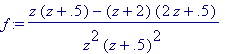
> f:=(z*(z+0.5) - (z+2)*(2*z+0.5) ) / (z^2*(z+0.5)^2 );

> rootlocus(f, z, -5..5, style=line, thickness=3);

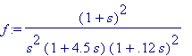
> f:=(1+s)^2/(s^2*(1+4.5*s)*(1+0.12*s)^2);

> rootlocus(f, s, -5..5, style=point);

>

>

2D

>

> coordplot(logarithmic,labelling=true, color=[black,black], linestyle=[1,2]);

>

>

> coordplot(polar, [0..1,0..7*Pi/4], labelling=true,
grid=[5,8], linestyle=[1,2],scaling=constrained);

> plot(phi, phi=0..2*Pi, coords=polar, color=black);

>

3D

> with(plots):

> r:=sin(phi) * cos( Pi/2 * sin(phi)*cos(theta) );

> plot3d( r, theta=0..2*Pi, phi=0..Pi,
style=patch, scaling=constrained, orientation=[-15,53],
grid=[35,35],coords=spherical );

> plot3d( 2+sin(z), theta=0..2*Pi, z=0..10, grid=[25,25],
orientation=[45,71], coords=cylindrical, style=patch);

> coordplot3d(cylindrical, [0..2,0..7*Pi/4, -1..1], orientation=[-13,49]);

>

>

>

Ungleichungen (2D)

> with(plots):

>

y-x/5<4 wird in Maple 6 falsch gezeichnet!

> inequal( { x+y>=-1, x-y/2<=1, y-x/5<4}, x=-5..4, y=-2..5,
optionsfeasible=(color=grey),
optionsclosed=(thickness=3),
optionsopen=(linestyle=3, thickness=1),
optionsexcluded=(color=white),
axes=normal );

>

>

>

> inequal( { y<x/5+4}, x=-5..4, y=-2..5,
optionsfeasible=(color=grey),
optionsclosed=(thickness=3),
optionsopen=(linestyle=3, thickness=1),
optionsexcluded=(color=yellow),
axes=normal );

>

>

implicitplot3d

> with(plots):

> implicitplot3d( x^2+y^2+z^2=1, x=-1..1, y=-1..1, z=-1..1,

> grid=[10,10,10], scaling=constrained);

> implicitplot3d(

> z+sqrt(x^2+y^2)-sin(y^2+z^3)=0,

> x=-2..2, y=-2..2, z=-2..2,

> grid=[20,20,10], orientation=[18,83],

> style=wireframe, color=black);

>

>

polyhedraplot

> with(plots):

> polys:=array([tetrahedron,octahedron,hexahedron,dodecahedron,icosahedron]):

> seq( polyhedraplot([2.5*n^1.6,n,n/3],

> polytype=polys[n], polyscale=1.5+n*0.7),

> n=1..5):

> display( [%], scaling=constrained, orientation=[-126,56], style=patch);

>

>

> restart:

> with(plots):

Warning, the name changecoords has been redefined

> animate( sin(x+phi), x=-1..8, phi=0..2*Pi, frames=30);

> animate3d( sin(sqrt(x^2+y^2)+phi), x=-6..6, y=-6..6, phi=0..2*Pi-2*Pi/15,
style=patch, frames=15);

> data:=[]:

> for i from 1 to 10 do

> phi:=2*Pi/10*i:

> data:=[op(data),

> tubeplot( [-t^1.5/5,3*cos(t+phi),3*sin(t+phi)], t=0..8*Pi, radius=t/8,

> scaling=constrained,grid=[60,15]) ]:

> od:

> display(data, insequence=true, orientation=[107,56]);

>

>