Leseproben:
Der harmonische Oszillator, quantenmechanisch
Beitrag zur Fortbildung Quantenphysik 2003
Licht - Quanten |
Quantenoptik für Amateure
Leseproben:
![]() Matrixoptik | Harmonischer
Oszillator | Quantisierung
des em. Feldes
Matrixoptik | Harmonischer
Oszillator | Quantisierung
des em. Feldes
Der harmonische Oszillator spielt auch in der Quantenphysik eine wichtige Rolle. Das quadratische Potential kommt zwar in der Realität nicht vor, ist aber eine bequeme Näherung für ein Potential mit einem Minimum, in der sich die Zustände (Lösungen der Schrödingergleichung) geschlossen berechnen lassen. Das Modell eignet sich nicht nur für den Vergleich der klassischen und quantenmechanischen Beschreibung der "harmonischen Schwingung eines Teilchens", sondern hat eine zentrale Bedeutung bei der Quantisierung des elektromagnetischen Feldes.
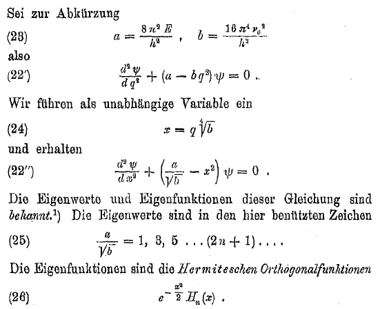
Schrödinger schreibt 1926 in seiner zweiten Mitteilung zu "Quantisierung als Eigenwertproblem":
Zur Behandlung dieses Themas im Zeitalter des Computers hier ein
Auszug aus einem Maple-Worksheet (2003):
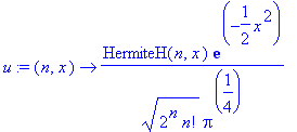
Stationäre Lösung der Schrödingergleichung für den harmonischen Oszillator (sigma=1, HermiteH(n,x) sind die Hermitepolynome)
| > | u:=(n,x)->1/sqrt(2^n*n!)*Pi^(-1/4)*HermiteH(n,x)*exp(-x^2/2); |
Die Energieniveaus sind diskret und äquidistant. Der Grundzustand hat nicht
die Energie Null. In Einheiten h*f (h= Wirkungsquantum, f = Frequenz des
(klassischen) Oszillators):
| > | E:=n->n+1/2; |
![]()
Potential ("Federkonstante" = 1):
| > | V:=x->x^2/2; |
![]()
| Darstellung für n = 3 Realteil der Wahrscheinlichkeitsamplitude (zur Orientierung ist immer das Potential mit eingezeichnet): |
| > | plot([u(3,x)+E(3),E(3),V(x)],x=-4..4,color=[red,blue,black]); |
![[Maple Plot]](images/harmosztk4.gif)
Betragsquadrat der W-Amplitude = Wahrscheinlichkeitsdichte
| > | plot([u(3,x)^2+E(3),E(3),V(x)],x=-4..4,color=[red,blue,black]); |
![[Maple Plot]](images/harmosztk5.gif)
Vergleich mit der klassischen Wahrscheinlichkeits-Verteilung
Klassische Wahrscheinlichkeitsdichte
| > | rhoklass:=n->1/(Pi*sqrt((2*E(n)-x^2))); |
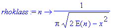
| > | int(rhoklass(13),x=0..sqrt(2*E(13))); |
![]()
Die Wahrscheinlichkeit, das Teilchen auf einer Hälfte der Schwingung anzutreffen, ist also 1/2 (nicht nur für n = 13 :-).
Vergleich der
W-Dichten für eine bestimmte (scharfe) Energie:
| > | plot([3*rhoklass(7)+E(7),3*u(7,x)^2+E(7),E(7),V(x)],x=-5..5,0..12,color=[green,red,blue,black],thickness=2); |
![[Maple Plot]](images/harmosztk8.gif)
Im Gegensatz zur klassischen W-Dichte (grün) oszilliert die
quantenmechanische (rot). An manchen Stellen ist sie sogar Null wie bei einer
stehenden Welle. Darüberhinaus
"hält sich das quantenmechanische Teilchen nicht an die Energieerhaltung", sondern
tunnelt an den klassischen Umkehrpunkten (Schnittpunkt von blau mit schwarz)
über den "erlaubten Bereich" hinaus.
Das sind doch gravierende Unterschiede der beiden Beschreibungen!
Allerdings haben wir bisher nur stationäre Zustände untersucht, bei denen sich nichts bewegt. Wir berücksichtigen zunächst die Zeitabhängigkeit der stationären Zustände:
Zeitabhängigkeit
| > | psi:=(n,x,t)->u(n,x)*exp(-I*E(n)*t); |
![]()
Im Gegensatz zum klassischen Oszillator ändert sich die Frequenz und Schwingungsdauer des Zustandes mit der Energie.
| > | T:=n->2*Pi/E(n); |
![]()
Animation des Realteils der Zustandsfunktion
| > | display([seq(plot([evalc(Re(psi(3,x,t)))+E(3),E(3),V(x)],x=-4..4,color=[red,black,blue],thickness=2),t=seq(T(3)*i/50,i=0..49))],insequence=true); |
![[Maple Plot]](images/harmosztk11.gif)
Das ist nur die halbe Wahrheit, denn die Zustandsfunktion ist komplex (Realteil noch oben, Imaginärteil nach hinten):
| > | display([seq(spacecurve([x,5*evalc(Im(psi(3,x,t))),5*evalc(Re(psi(3,x,t)))],x=-5..5,axes=frame,numpoints=250,shading=ZHUE,thickness=2),t=seq(T(3)*i/48,i=0..47))],insequence=true); |
![[Maple Plot]](images/harmosztk12.gif)
Nun gut "die Zustandsfunktion rotiert". Nach wie vor ist aber keine klassische Schwingung in horizontale Richtung zu sehen. Das ändert sich aber, wenn man Zustände überlagert:
Überlagerung von Zuständen
Grundzustand und "erste Oberschwingung" mit gleichem Gewicht:
![[Maple Plot]](images/harmosztk13.gif)
| > | display([seq(plot([evalc(abs(psig))^2+Eq,Eq,V(x)],x=-4..4,color=[red,blue,black],thickness=2),t=seq(2*Pi*i/48,i=0..47))],insequence=true); |
![[Maple Plot]](images/harmosztk14.gif)
Aha! Mit etwas Phantasie kann man sich vorstellen, dass hier ein Teilchen horizontal schwingt. In den Umkehrpunkten hält es sich länger auf als im Nulldurchgang. Gibt es für die Überlagerung der Zustände (stationäre Eigenfunktionen) eine Gewichtung, die der klassischen Vorstellung etwas näher kommt?
Poissonverteilung für kohärente Zustände (Schrödinger: "Der stetige Übergang von der Mikro- zur Makromechanik")
Gewichte der Amplituden (Wurzel aus Poissonverteilung mit Mittelwert λ^2):
| > | af:=n->lambda^n/sqrt(n!)*exp(-lambda^2/2); |
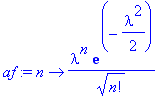
Histogramm der Gewichte (bis zu n = 8)
![[Maple Plot]](images/harmosztk16.gif)
Damit lässt sich tatsächlich ein Paket aufbauen. Das Betragsquadrat sieht so aus...
| > | display([seq(plot([Eq,2*psigabs+Eq,V(x)],x=-5..5,0..8,color=[blue,red,black],thickness=[1,2,2]),t=seq(2*Pi*i/96,i=0..95))],insequence=true); |
![[Maple Plot]](images/harmosztk17.gif)
... und schwingt horizontal. Fügt man noch weitere Oberschwingungen hinzu, schwingt ein Gaußpaket ohne Formänderung horizontal:


Aber Vorsicht mit Analogien! Insbesondere der Vergleich mit einer Kugel, die im "Schwerefeld auf einer Parabelbahn rollt", ist nicht angebracht, siehe " Das Märchen vom harmonischen Oszillator im Schwerefeld".
Und hier ist wieder die volle Wahrheit (n = 8):
| > | display([seq(display([seq(pzeig(xx,t),xx=seq(k,k=seq(j/5,j=-25..25))),spacecurve(psigspace(x,t),x=-5..5,axes=frame,numpoints=250,shading=ZHUE,thickness=2)]),t=seq(4*Pi*i/96,i=0..95))],insequence=true); |
![[Maple Plot]](images/harmosztk18.gif)
Wenn man die Zustandsfunktion mit Real- und Imaginärteil darstellt, wird deutlich, was sich hinter den Kulissen abspielt. Die komplexen Zahlen sind durch "Zeiger" (schwarze Linien) dargestellt.
Dabei kommt ein Zeiger so zustande (exemplarisch):
| > | display([seq(display([plot([[0,0],seq(p[i],i=1..nmax)],color=red),plot([p[nmax],[0,0]],color=black)],thickness=2),t=seq(4*Pi*i/96,i=0..95))],insequence=true); |
![[Maple Plot]](images/harmosztk19.gif)
Hier sind noch einmal die gewichteten Eigenfunktionen (Poissonverteilung):
| > | plot([seq(av[i]*psiv[i],i=1..nmax)],x=-5..5); |
![[Maple Plot]](images/harmosztk20.gif)
Etwas übersichtlicher auf der Höhe der Energieen abgetragen
| > | plot([seq(av[i]*psiv[i]+Ev[i],i=1..nmax),V(x),seq(Ev[i],i=1..nmax)],x=-5..5,0..10); |
![[Maple Plot]](images/harmosztk21.gif)
Zusammenfassung:
Die "klassische Bewegung" entsteht in der quantenmechanischen Beschreibung erst durch Überlagerung von Zuständen (die es beim klassischen Oszillator nicht gibt).
Die Bewegung hat dann die Differenzfrequenz benachbarter Zustände (wie bei der Abstrahlung im Atom). Die Besonderheit des quantenmechanischen Oszillators ist, dass diese Zustände äquidistant liegen (Energie oder Frequenz) und somit die Fourierreihe die Differenzfrequenz benachbarter Zustände als Frequenz des klassischen Oszillators liefert.
Die Vorstellung, dass die quantenmechanische Beschreibung die Amplitude des klassischen Oszillators (direkt) quantisiert, ist falsch, denn der Mittelwert der Verteilung kann alle Werte annehmen.
Siehe auch: Schrödingers Oszillator | harmonischer Oszillator, klassisch | Atomarer Dipol
Zurück zum Inhalt (Fortbildung zur QPh 2003, Mathematische Behandlung der Schrödingergleichung)
Moderne Physik mit MapleHOME | Projekte | Physik | Elektrizität | Optik | Atomphysik | Quantenphysik | Top