Superradiance 

A short note 

1. Neoclassical

As explained in Über die spontane Emission von Photonen, the emission of a photon, i.e. the transition of a single atom from a higher to a lower energy level, can be described by the logistic equation:

Unfortunately, individual atoms and their states and transitions are not easy to observe. How about a "macroscopic atom", i.e. a "suitable collection of N identical atoms"?
Then one would - purely theoretically - only have to replace the 1 by N in the above equation for ρ_gg. The logistic equation is then

>

(1)

For comparison with the quantum-optical description (see below), the designations (and the sign) were adapted to the notation by Mandel and Wolf [MaWo]. This DE has the general solution

>

(2)

or with t0 as time shift

>

(3)

which can also be written as a tanh function

>

Compared to the standardized solution, not only does the amplitude change, but also the proportionality constant in the exponent by a factor of N. The radiated power then is

(4)

Here is an illustration for k=0.5, t0=2 and N=2,5,10 (red: state, blue: radiation):

From this "neoclassical" treatment alone, it follows that the radiated power increases with N², which is considered a characteristic of superradiance.

2. Quantum optical description

In "Optical Coherence and Quantum Optics", L. Mandel and E. Wolf, S. 844 (16.6-14) [MaWo] one finds the differential equation

>

(8)

where y(t) = |c₂(t)|² is the excited state density, N is the number of atoms and A is the "Einstein coefficient". This DE has the general solution

>

(9)

However, this means that the density of the excited state is greater than 1 for negative times 

>

(10)

and infinite for a single atom. But that can be remedied if, like [MaWo], you only look at positive times and set the density at time 0 to 1:

>

(11)

The solution curves for N=1..10 look like this

3. Comparison neoclassic - quantum optics

The above quantum-optical solution (11) refers to one atom. To compare it with the neoclassical solution, it has to be multiplied by the number N of atoms:

(13)

With

(14)

one then gets (red: "quantum optical", blue: "neoclassical")

>

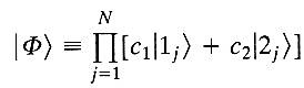
The figure on the right makes the behavior of the solutions for t<0 particularly clear.

That is, a single atom "decays" exponentially, but as soon as just a second atom is added, both "decay" logistically. This is of course due to the approach taken. The state of the "N-atom system" is set as a product state of superposition states ([MaWo] p. 841)

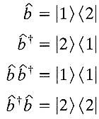
with identical time-dependent amplitudes c for all atoms, resulting in "cooperative atomic radiation" [MaWo]. The condition for this is a "suitable accumulation" (see above), i.e. the extent of the accumulation of atoms must be significantly smaller than the wavelength of the radiation, which is of course coherent when all atoms oscillate in phase.

One forms with the "ladder operators" b ([MaWo] p. 744, (15.2-14)): 

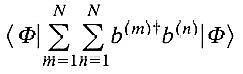
the expectation value ([MaWo] S.842, (16.6-10))

what means (with b⁺b = |2><2|), that for m=n (i.e. in a single atom) paradoxically no transitions take place.

It remains to be mentioned that in [MaWo] on pages 845-847 for N ≫ 1 an approximate solution is worked out that is identical to the neoclassical result.

© März 2022, Dr. Michael Komma (VGWORT)

Literatur:  [MaWo] Optical Coherence and Quantum Optics, L.Mandel and E.Wolf (Cambridge University Press 1995, reprinted 2008).

Links:  Spontane Emission | Kaskade | Photogalerie | Photonenemission | Weisskopf-Wigner | Ensemble-Individuum | Minev Quantum Jump

HOME | Fächer | Physik | Elektrizität | Optik | Atomphysik | Quantenphysik | Top